
Data Analysis with SQL: Exploring Window Functions

I don't write about SQL enough, but I probably should. Anyone who knows Python should also strive to learn SQL, and vice versa. Tools don't operate in isolation. Many companies have a technology stack that integrates multiple tools. This means that when they are looking for talent, they are seeking individuals who can work with a variety of tools. For those interested in working with data, both Python and SQL are essential tools to learn.
In this article, we are going to dive into one of the most popular subjects in SQL: window functions. Window functions provide a powerful way to perform calculations across a set of table rows that are related to the current row. Unlike aggregate functions, which collapse rows into a single result, window functions retain individual rows while performing calculations across a group or "window" of rows. They are particularly useful for tasks like calculating running totals, rankings, moving averages, or cumulative sums. Let's look at some of the window functions and how we can use them in data analysis.
ROW_NUMBER
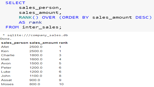
The first window function that we are going to look at is the ROW_NUMBER() function. Let’s say we want to rank the sales table by the sales_amount column. That is, we want every sales_person in the table to be given a rank based on the sales they brought in; we can use the ROW_NUMBER() function. The function ROW_NUMBER() assigns a unique, sequential integer to each row based on the order defined in the OVER clause. The numbering starts at 1 and increments by 1 for each row. See example below:

Let’s break down what is happening here. All window functions will have the OVER keyword. So whenever you see this word in a query, just know that there is a window function. Imagine you have a list of sales data for different salespersons. You want to rank the salespersons based on their total sales, from lowest to highest. This is what is happening here. Here the OVER clause defines how the window function should operate. Basically, to rank all rows based on the sales_amount column The rank should be ordered by the sales_amount column in descending order. This means that the salesperson with the highest sales amount will be given a rank of 1.
The ROW_NUMBER() function assigns a sequential number to each row based on the sales values. It will assign the person with the highest amount a rank of 1 and the next person a rank of 2, just like that. You can see the ranking in the rank column. Notice that Afet and Ken both achieved a sales amount of $2500 (which is a tie), and they have been given a rank of 1 and 2 even though the sales amount is equal. This is because of the behavior of the ROW_NUMBER function. This function will assign consecutive numbers, even if there are ties.
Tackle Data Analysis Projects with Confidence
Start your 2025 strong by acquiring the skills required to tackle data analysis projects with Python. Learn the important Python libraries used in data analysis. This book gives you the hands-on learning experience that you need to take your skills to the next level. Start your 50-day journey now to start 2025 strong. 50 Days of Data Analysis with Python.

Other Resource
Master Python fundamentals by doing challenges with: 50 Days of Python: A Challenge a Day
RANK
Unlike the ROW_NUMBER() function, which assigns consecutive numbers even when there is a tie, the RANK() function will assign the same number to ties. You can see below that those that achieved the sales of 2500 have been assigned a rank of 1. Once there is a tie, the RANK() function will skip a number. This means that after a rank of 1, the next one will be 3. So basically, RANK() introduces gaps in the ranking sequence when there are ties. See below:
So when should you use the RANK function? Let’s say you want to identify the top-selling salespeople, and you want to ensure that the salespeople with a tie are assigned the same value, and you don’t mind the gaps in the ranking; then use the RANK function. Let’s say we want to identify all salespeople who brought in the most sales (ranked number 1). Here is how we can use the RANK function:

Here, because we are using the RANK() function, the top-selling persons have been assigned the same rank. So we are able to retrieve both names. If we had used the ROW_NUMBER() function, then only one name would have been retrieved because the two top people would have been assigned different ranks even though they have achieved the same sales amount.
DENSE_RANK
DENSE_RANK() works similarly to the RANK() function; the only major difference is that after a tie, it does not introduce gaps. See below:

You can see here that after the tie of ranks 1 and 5, there are no gaps in the sequence.
PARTITION
So far, when creating ranks, we have treated the whole dataset as one group. However, we can also divide the dataset into subsets of partitions and rank the data in each partition. Let’s look at a practical example. We want to know who the top salesperson is per country. If there is a tie, we want both sellers to be retrieved, and we don’t want gaps in the ranking. We can partition the data by country (that is, create two subsets, one for sellers in South Africa and another for sellers in Turkey) and rank the seller in each partition by the sales amount using DENSE_RANK(). See below:

You can see below that we have partitioned the data by country. We now have a ranking for sellers in South Africa and a ranking for sellers in Turkey. We can easily see who are the top sellers in each country. Since we are using DENSE_RANK(), sellers who are tied in each country have been given the same rank (Afet and Ken in Turkey), and there are no gaps in the ranks. To retrieve the names of the top sellers, we can convert the above query into a Common Table Expression (CTE) and then query it using the main query. See below:

So we have two top sellers in Turkey (tie) and one top seller in South Africa.
Running Totals
When we use an aggregate function with the OVER clause, that function becomes a window function. We use the SUM() window function to calculate cumulative values. Let’s look at another example. Let’s say we want to know how the sales amount increased over time in each country. We can partition the data by country and calculate the cumulative sum within each partition. See the query below:
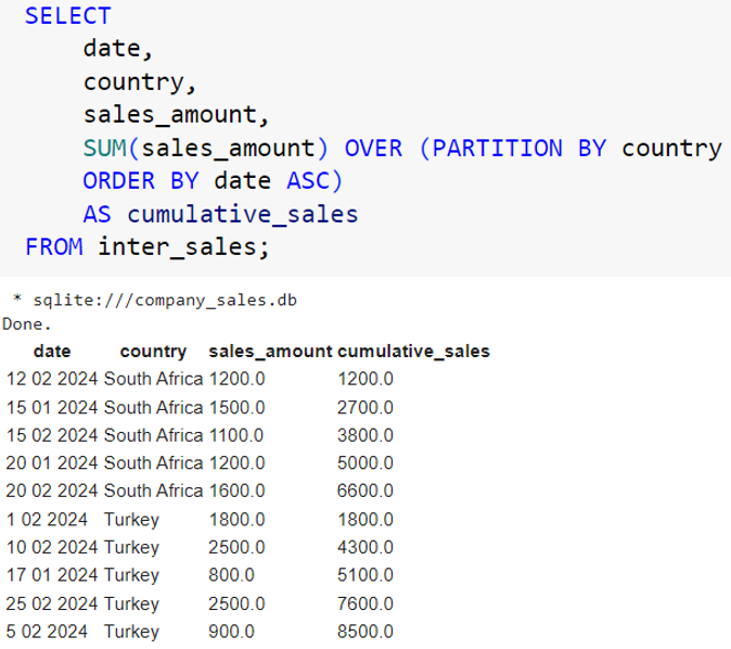
In this query, we partition the data into subsets (partitions) based on country. The cumulative sum is calculated separately for each country. The SUM() function accumulates the sales_amount over time, giving the running total of sales per country. Within each partition (country), the sales data is ordered by the date column in ascending order. The cumulative sum is calculated in this order. This type of query can be useful for tracking sales growth over time for each country, providing insights into country-specific sales trends.
We can do similar things with the AVG function. We can use it as a window function to calculate the cumulative average of sales over time for each country.

Here, we are calculating the cumulative (running) average of sales over time for each country. This is saved in the cumulative_avg_sales column.
Moving Average (Using a Window Frame)
We can also calculate a moving average over a specified number of rows using window frames. For example, we can calculate a 3-day moving average of sales for each country by defining a 3-day window frame. See below:

In this query, ROWS BETWEEN 2 PRECEDING AND CURRENT ROW defines the window frame to include the current row and the two preceding rows. This means for each row, the average is calculated by using the sales amount of the current row and the two preceding rows, effectively giving us a 3-day moving average. For example, the moving average value of 1300 for South Africa is calculated from 1600.0 as the current value and 1200 and 1100 as the two preceding rows.
Final Thoughts
We can keep going and talk about other window functions, but we will stop here. I guess you have seen the power of window functions. Whether you're working with sales data, financial time series, or any other type of relational data, window functions can help you find insights in the data and help you make data-driven decisions with confidence.This article has provided an introduction to some of the key window functions in SQL. However, the possibilities are vast. I encourage you to experiment with these functions, explore different window frames, and discover how they can be applied to solve a wide range of data analysis challenges. Thanks for reading.