
50 Days of Data Analysis: Analyzing Data with NumPy

Master the Skills Required in Data Analysis and Machine Learning
Start a transformative journey with "50 Days of Data Analysis with Python." Dive into the world of Python libraries used in data analysis and machine learning, conquer real-world scenarios, and master the art of data analysis. This immersive resource offers 300+ hands-on challenges to help you become a proficient data analyst. (Click Here.)
Introduction
NumPy is one of the most important libraries in data analysis. It provides powerful tools for handling numerical data efficiently. However, since it is so huge, it can be challenging for beginners to identify the most essential functions to master.
When writing 50 Days of Data Analysis with Python: The Ultimate Challenge Book for Beginners, my goal was to introduce learners to the most critical functions in Pandas, NumPy, Seaborn, Matplotlib, and Scikit-learn that are widely used in real-world data analysis.
Today, we’re diving into NumPy, specifically tackling challenges from Day 15 of 50 Days of Data Analysis. These challenges focus on filtering data operations, demonstrating how NumPy can be used to extract insights from data. Let’s get started!
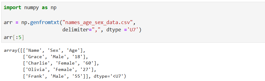
1. Your task is to import the CSV file using NumPy's genfromtxt() function.
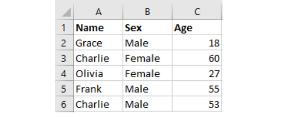
Most of the time, we import CSV data using pandas. However, this challenge challenges you to import CSV data using NumPy’s genfromtxt() function, which is a fundamental skill for data analysts. By tackling this challenge, you will learn how to handle structured data using NumPy (deal with delimiters and specify data types). This is the data that we are required to import:
In the code below, the delimiter parameter specifies that the data be separated by commas. The dtype parameter set 'U7' specifies that the column should be treated as Unicode strings of length up to 7 characters.
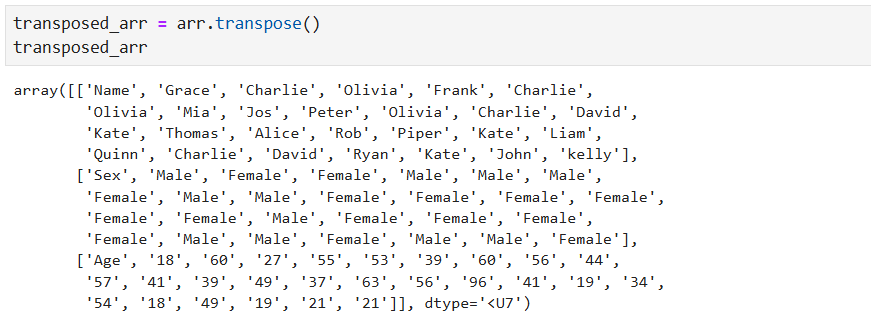
a. Transpose the array.
Transposing arrays is a useful operation in data analysis for restructuring data to better suit analysis needs such as matrix calculations, correlation analysis, or plotting, even visualizations.
In NumPy, you can use the transpose() method to transpose an array. Transpose swaps the axes of an array.
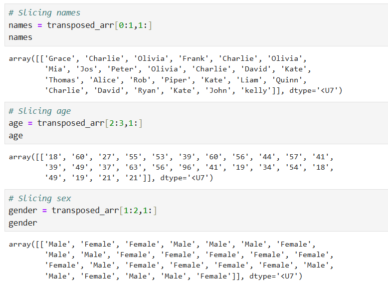
b. Using slicing, create three arrays: an array of all the names column, an array of the age column, and an array of the gender (sex) column from the array.
This is the second part question that introduces slicing techniques in NumPy, which are essential for extracting specific subsets of data from arrays. For data analysts, mastering slicing data is one of the most important skills to have. This skill is needed for tasks such as isolating variables (e.g., names, ages, genders) for statistical analysis or visualization.
We want to extract names, age, and gender. Let's breakdown what is happening in the first slice. The names are in the first row of the transposed_arr. The first row is sitting at index 0. To meet the requirement, we have to carry out a row and column slice. Here is the breakdown:
Row Slice: 0:1
0: Start at row index 0 (the first row).
1: Stop before row index 1 (so only row 0 is included).
This row slice will select only the first row but keep it as a 2D array (shape (1, n)).
Column Slice: 1:
Starts at column 1 (skipping column 0, which contains the header "Name").
1: means "include all columns from index 1 onward."
This will select all columns except the first one (column 0). This breakdown is for the first slice. You can use the same logic to slice age and gender arrays. The most important thing is to understand the structure of the transposed array.
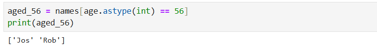
2. Using NumPy, write code that returns all the names of people who are 56 years old.
This question is quite straightforward. It introduces boolean indexing, a powerful technique for filtering data based on specific conditions, which is common in data analysis for targeting particular subsets of data.
To answer the question, we will create a boolean mask using (names[age == 56]) to filter the names array to return only the names where the corresponding age is 56. The True values in the boolean mask indicate rows in the age array where the age value is exactly 56. For instance, if names = ["Alice", "Bob", "Charlie"] and age = [25, 56, 30], age == 56 will produce [False, True, False], this would return ["Bob"]. Here is the query below:
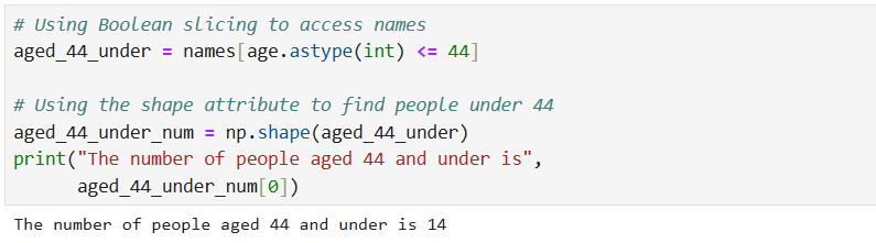
3. How many people are aged 44 or under?
This question asks that we calculate the counts of people that are 44 years old or under. Counting a segment of data is a frequent task in data analysis.
If you successfully tackled question 2, then you must have an idea of how to tackle this one. Like in the previous question, first, we create a boolean mask where True indicates rows in the age array where the age value is less than or equal to 44, and False otherwise. We then use the shape() function to count the number of True values. The shape() returns a tuple. To access the element in the tuple, we use indexing (aged_44_under_num[0]). Here is the query below:
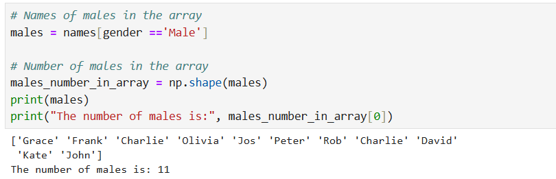
4. Write another code snippet to return an array of all the males in the dataset. How many males are in the dataset?
This question has two parts: filtering data by categories (gender) and counting occurrences of that gender (basically counting the number of males we have). This may come in handy when you are doing demographic analysis.
To solve the question, first we filter the gender array to return an array of male names using (males = names[gender == 'Male']). This part of the code: gender == 'Male' creates a boolean mask where True indicates rows in the gender array where the value is "Male," and False otherwise. This mask will be used to filter the names array to include only the names where the boolean mask is True. To count the number of names in the males array, we use the shape() function. The shape() function returns an array (n, ), where n is the number of elements (i.e., the number of males). Since np.shape(males) returns a tuple, [0] extracts the first (and only) element, giving the count of males. Here is the query below:
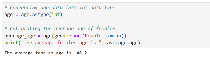
5. Calculate the average age of all the females in the table.
This question reinforces skills in filtering data by categories and using statistical functions to calculate average values. These skills are critical for many tasks in data analysis.
First, we are going to convert the age array into an integer data type since we want to perform arithmetic operations on the array. We are using the astype() method to convert age. Next, we use boolean indexing to create a boolean mask where True indicates rows in the gender array where the value is "Female" and False otherwise. We then use these True values to extract the ages corresponding to females. The mean() method is used to calculate the average age of all females. Here is the query below:
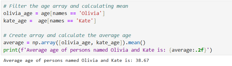
6. Calculate the average age of people named Olivia and Kate.
This question is about combining multiple conditions, a common requirement in data analysis.
To answer this question, first we need to access the ages of Olivia and Kate. We are going to create a boolean mask for each value (Olivia and Kate). The boolean mask will be used to retrieve the ages of these two individuals. We save these values to two variables (olivia_age and kate_age). Step two is to create an array from these two values and use the mean() function to calculate the average age. Here is the code below:
Final Thoughts
When a mechanic faces a problem, their first step is to observe and diagnose the issue before selecting the right tool for the job. The ability to choose the right tool is a skill honed over time through experience.
The same principle applies to data analysis. First, you learn the essential NumPy functions used in data analysis. Then, you develop the ability to select the right function for each problem. This is a skill that takes time and practice to master. For example, understanding Boolean indexing is one thing; applying it effectively in a data analysis scenario and perhaps combining it with statistical calculations is another. That’s why hands-on practice is crucial.
I hope these challenges have given you a glimpse into the power of NumPy and, more importantly, reinforced the value of incorporating challenges into your learning journey.
There are more challenges in the 50 Days of Data Analysis. Thank you for reading!